Published on
June 5, 2026


ARIMA (AutoRegressive Integrated Moving Average) models are statistical tools for forecasting time series data, like revenue trends. They combine three components: AutoRegressive (AR) for past values, Integrated (I) for trend removal, and Moving Average (MA) for error adjustments. By analyzing historical revenue data, ARIMA helps businesses predict future performance with transparency and accuracy.
Key points:
Advanced methods like SARIMA add seasonal adjustments, while SARIMAX incorporates external factors like marketing campaigns or economic shifts. Regular updates, validation, and monitoring ensure ARIMA remains effective for financial planning, budgeting, and decision-making.
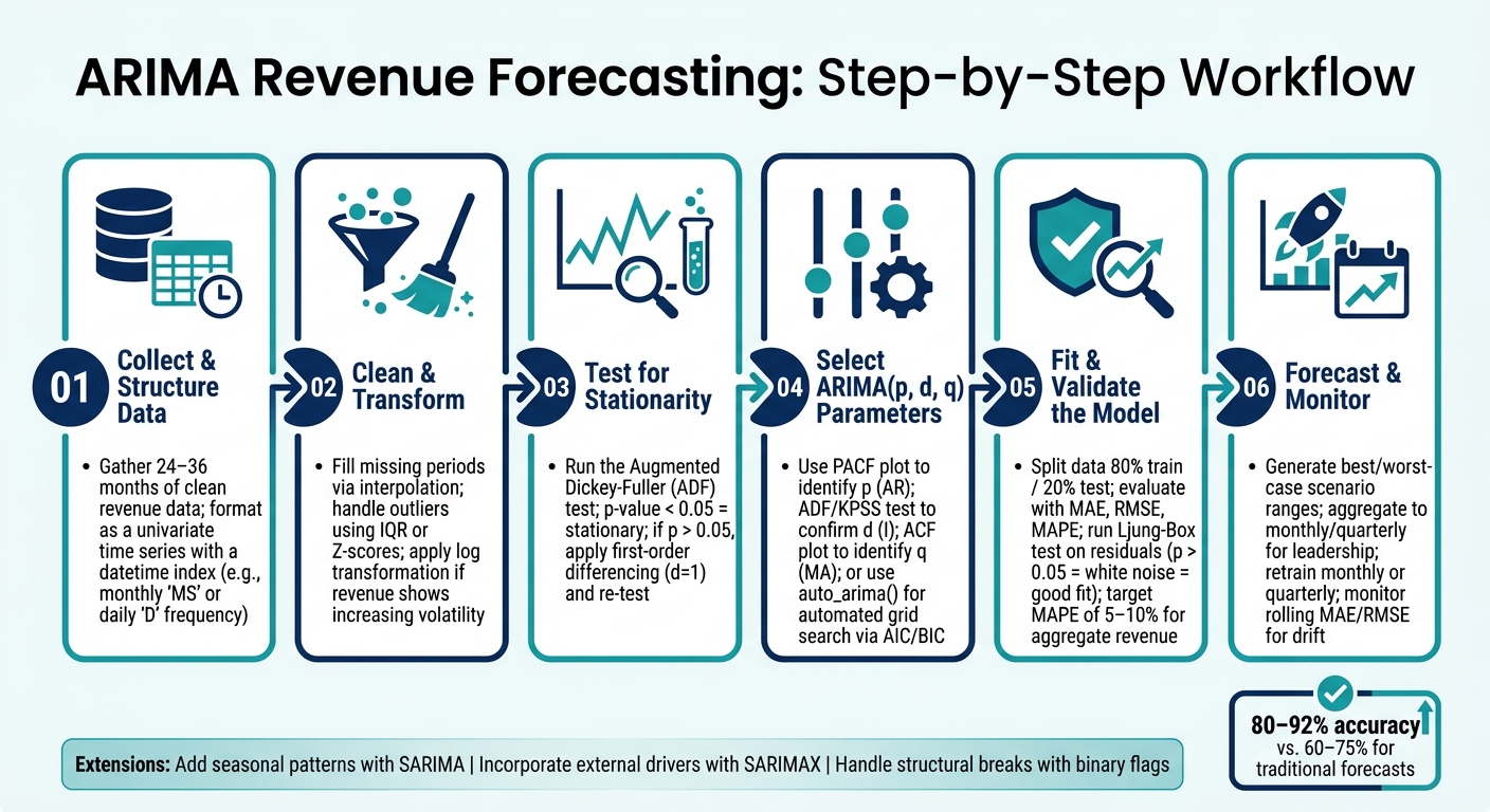
ARIMA Revenue Forecasting: Step-by-Step Workflow
Accurate forecasts start with well-prepared data. As the Prospeo Team wisely notes:
"Your forecast is only as good as your pipeline data. Garbage in, garbage out - no algorithm fixes bad inputs." [3]
Before diving into model parameters, your revenue data needs to be properly structured, cleaned, and stationary.
ARIMA models work with a univariate time series - a single column of revenue figures arranged in chronological order at regular intervals. To prepare your data:
Monthly_Revenue_USD).'MS' for monthly data or 'D' for daily data.If your accounting system provides raw transactional data with multiple entries per day, you’ll need to summarize these into consistent time intervals. Tools like QuickBooks or NetSuite often allow you to export revenue summaries (e.g., monthly or weekly), which can serve as your starting point for modeling.
Once your data is structured, focus on cleaning it. The two most common issues you’ll encounter are missing values and outliers.
If your revenue shows increasing volatility due to growth over time, consider applying a log transformation. This stabilizes variance and prevents the model from over-emphasizing recent high-revenue periods [2][3].
After cleaning and transforming your data, the next step is to test for stationarity.
ARIMA models require the data’s statistical properties - such as mean, variance, and autocorrelation - to remain stable over time [2]. If your data trends upward or shows significant changes over time, it violates this assumption. The solution? Differencing - subtracting each observation from the one before it to remove trends.
To confirm stationarity, use the Augmented Dickey-Fuller (ADF) test. A p-value below 0.05 means the data is stationary and ready for modeling. If the p-value is higher, apply differencing and re-test. For example, in a 90-day forecasting project, analyst May Cooper found the raw revenue data had an ADF p-value of 0.32 (non-stationary). After applying first-order differencing (d=1), the p-value dropped to 0.00, confirming stationarity [1].
Important Note: Avoid over-differencing. Stop as soon as the data becomes stationary. Signs of over-differencing include increased standard deviation or negative lag-1 autocorrelation. Over-differencing introduces unnecessary noise into the series [8].
Once your data is stationary, you’re ready to move on to building and validating your ARIMA model. Clean, structured, and stable data is the foundation for accurate forecasting.
Once your data is stationary, it's time to construct the ARIMA model. As Let's Data Science explains:
"Think of ARIMA as a recipe with three ingredients you mix in different proportions." – Let's Data Science [2]
This section guides you through selecting the right parameters and ensuring your model is ready for forecasting.
Each ARIMA parameter plays a distinct role in interpreting historical revenue data:
| Parameter | Role in Revenue Modeling | Identification Tool |
|---|---|---|
| p (AR) | Reflects long-term momentum or inertia in revenue | PACF plot spikes |
| d (I) | Removes trends to stabilize the data's mean | ADF / KPSS tests |
| q (MA) | Accounts for short-term fluctuations or random shocks | ACF plot spikes |
The p parameter determines the influence of past revenue values on future predictions [2] [9]. The d parameter, identified during stationarity testing, represents the number of differences applied to stabilize the series. Lastly, the q parameter helps smooth out short-term surprises by factoring in previous forecast errors [2] [9]. It's worth noting that setting the d value higher than 2 can often introduce unnecessary noise [2] [9].
After determining the differencing order (d), ACF and PACF plots help identify appropriate values for p and q. A sharp drop-off in the PACF at lag k suggests using p = k, while a similar cutoff in the ACF suggests q = k. If both plots show a gradual decay, you may need to include both AR and MA components in the model.
For automation, Python's pmdarima.auto_arima function can perform a grid search to find the best (p, d, q) combination based on metrics like AIC or BIC. In R, the forecast::auto.arima function employs the Hyndman-Khandakar algorithm to achieve the same goal [7] [10]. However, automated tools should be used as a starting point - always inspect residuals manually to ensure the model is sound.
One critical consideration is the inclusion of a constant term. If d = 1 and a constant is included, the long-term forecast will follow a linear trend. For d = 2, omit the constant to avoid introducing a quadratic trend [7]. After fitting the model, validate its performance before deploying it for forecasting.
Fitting the model is just the beginning; validation ensures it performs well on unseen data. A common practice is to split the historical revenue data into a training set (about 80%) and a test set (20%). Then, evaluate the model using error metrics like MAE, RMSE, or MAPE [1] [6].
Additionally, perform a Ljung-Box test on the residuals. A p-value above 0.05 suggests the residuals resemble white noise, indicating the model has successfully captured the underlying patterns in your data [1] [2] [9]. Check the residual ACF plot to ensure all spikes fall within the confidence bounds. For example, in a 90-day revenue forecasting project using 731 days of historical data, an ARIMA(1,0,0) model achieved an RMSE of 0.57 and a Ljung-Box p-value of 0.96 [1].
If the Ljung-Box p-value is below 0.05, it signals residual autocorrelation, and you may need to adjust p or q. Avoid over-complicating the model - if AR or MA coefficients approach 1 or –1, simplify the model by reducing p or q and comparing AIC values. In general, a simpler model that performs just as well is preferred [2].
Once you’ve validated your ARIMA model, you can take it further by incorporating advanced techniques to handle seasonal patterns, external drivers, and structural shifts. These enhancements make your forecasts more precise and aligned with real-world dynamics.
Standard ARIMA models often struggle with recurring seasonal trends, such as Q4 holiday sales spikes. That’s where SARIMA (Seasonal ARIMA) comes into play. SARIMA builds on ARIMA by adding seasonal parameters to the traditional (p, d, q) structure. Its full notation, (p,d,q)(P,D,Q)_m, includes seasonal components (P, D, Q) and a seasonal cycle length, m (e.g., m = 12 for monthly data or m = 4 for quarterly data) [11].
To pinpoint seasonal parameters, examine the ACF and PACF plots at seasonal lags - like 12, 24, or 36 for monthly data. For instance, a strong spike at lag 12 in the ACF often points to a seasonal MA(1) component [11]. By accounting for these seasonal effects, SARIMA ensures your model reflects recurring revenue cycles more effectively.
Revenue patterns are rarely shaped by internal factors alone. External drivers - like marketing campaigns, pricing changes, or broader economic shifts - can significantly influence outcomes. SARIMAX takes SARIMA a step further by incorporating these exogenous variables through the exog argument in statsmodels [12].
This method first regresses revenue against external factors and then applies ARIMA to the residuals. As Robert Nau, a professor at Duke University, explains:
"Variables which measure advertising or price levels or the occurrence of promotional events are often helpful in augmenting ARIMA models... for forecasting sales at the level of the firm or product." [14]
To make this work, ensure you have reliable future values for each exogenous variable [13]. Properly integrating these factors can tighten prediction intervals by explaining variations that might otherwise appear as noise [15].
Even with external variables, abrupt changes in revenue trends - like a new product launch, a major acquisition, or losing a key client - can disrupt your model. These structural breaks can distort trends and widen forecast intervals if left unaddressed [16].
To account for these shifts, use a binary flag in SARIMAX (0 before the break, 1 after) to adjust the intercept without discarding historical data. For more dramatic changes, consider building separate models for the periods before and after the break. Regularly monitoring rolling metrics like MAE and RMSE can help identify when such shifts occur, signaling the need for adjustments [16].
Running a single ARIMA model isn’t enough to meet the demands of a dynamic financial environment. The real advantage lies in creating a forecasting pipeline that automates the entire process - pulling in fresh revenue data, retraining the model, and generating updated forecasts on a regular schedule.
To set this up, connect your revenue data warehouse - whether it’s Snowflake, BigQuery, or another platform - to a Python script. Use libraries like pmdarima and statsmodels for tasks like automated stationarity testing and parameter selection through auto_arima(), which evaluates a manageable number of model combinations [2]. Incorporate rolling window cross-validation to simulate real-world conditions. Regular retraining, either monthly or quarterly, ensures the model stays in sync with evolving data patterns.
Once the pipeline is in place, the next step is continuous monitoring to ensure the model remains effective over time.
After launching your pipeline, keeping an eye on its performance is just as important as building it. Use the Ljung-Box test on residuals after each retraining cycle to check for emerging patterns. If new trends are detected, tweak the model parameters accordingly.
Accuracy metrics like MAPE (Mean Absolute Percentage Error) and systematic bias should be monitored closely. Even small errors in directional trends can significantly impact budgeting or hiring decisions. For context, aggregate revenue forecasts typically fall within a 5–10% MAPE range, while forecasts at the product-category level often range from 15–25% [3]. If your metrics stray outside these ranges, it could point to data quality issues, which are responsible for about 62% of forecasting errors in B2B settings [4].
By consistently evaluating performance, you can ensure your model remains a reliable tool for guiding financial strategies.
ARIMA forecasts offer more than just a single revenue figure - they provide a range of outcomes, from best-case to worst-case scenarios. This flexibility is invaluable for financial scenario planning. Teams can use these ranges to refine cash flow projections, foster transparent budget discussions, and assess risks more thoroughly.
To make forecasts actionable, aggregate daily or weekly ARIMA outputs into monthly or quarterly summaries before presenting them to leadership. Daily fluctuations can obscure trends, but smoothing the data helps align forecasts with budget targets and resource planning [5]. For example, Phoenix Strategy Group integrates this structured approach into regular FP&A cycles, linking forecasts to cash flow management, hiring plans, and board-level reporting. Similarly, in 2024, Walmart’s Global Tech team demonstrated the power of ARIMA at scale by combining ARIMA-based forecasts with hierarchical reconciliation across product levels, achieving a 3% to 40% improvement in APE over their previous methods [3].
ARIMA models offer U.S. mid-market companies a straightforward process for transforming 24–36 months of clean revenue data into actionable insights. This journey involves key steps like stationarity testing, parameter selection using tools like AIC and ACF/PACF, and walk-forward validation. The result? Better-informed decisions around staffing and budgeting [3][6].
ARIMA's strength lies in its dependability rather than its complexity. As the Prospeo Team aptly puts it:
"Time series sales forecasting isn't about finding the fanciest algorithm. It's about clean data, honest validation, and choosing the simplest model that meets your accuracy threshold." [3]
A 2026 Deloitte survey of 1,854 executives revealed that only 6% achieved AI ROI within a year. This highlights how simpler, fine-tuned models like ARIMA can often deliver quicker, more tangible value [3].
The real advantage comes from consistent use. Rolling forecasts, retraining, and residual checks ensure the model stays aligned with changing market dynamics. When expanded to include seasonal patterns or external variables using SARIMA or SARIMAX, the model becomes even more attuned to the factors driving revenue [1][6].
For teams at Phoenix Strategy Group, structured forecasting is a cornerstone of financial clarity. By tying quantitative revenue forecasts to cash flow management, board reporting, and strategic planning, businesses can create forecasts that are not only auditable but also actionable. This ARIMA-driven approach turns raw data into insights that support sound financial planning and long-term success.
ARIMA works well for short-term forecasting when dealing with stable, single-variable revenue data that doesn't have complex or multiple seasonal patterns. One of its strengths is how easy it is to understand and interpret.
However, if your data includes noticeable seasonal trends, SARIMA might be a better option. And if your revenue is impacted by external factors or involves non-linear dynamics, advanced methods like machine learning could provide more accurate predictions.
For growth-stage businesses, Phoenix Strategy Group specializes in helping evaluate and implement the most effective forecasting techniques.
To ensure your ARIMA revenue forecast model stays precise, it's important to update it frequently to account for shifting market dynamics. Incorporate walk-forward validation to retrain the model continuously as fresh financial data comes in. This method helps maintain the reliability of your forecasts over time. Phoenix Strategy Group offers financial advisory services, including data engineering and FP&A support, designed to help growth-stage businesses establish strong forecasting practices and scale efficiently.
When a one-time event disrupts your revenue trend, start by determining if it’s a recurring event, like holidays or promotions, or a rare anomaly. For recurring patterns, tweak your model to accommodate these predictable spikes. If the event hints at a lasting shift, investigate potential changepoints in your data. For major anomalies, evaluate whether your historical data remains applicable. If it doesn’t, consider using judgment-based adjustments or causal models to improve the accuracy of your forecasts.