Published on
January 6, 2026


State space models (SSMs) are reshaping financial forecasting by addressing the limitations of older methods like ARIMA. They excel in dynamic environments, handling non-stationary data, noise, and missing values with precision. By separating hidden system dynamics from observable data, SSMs provide more reliable and actionable forecasts. Tools like the Kalman Filter enable real-time updates, making these models especially useful for growth-stage companies managing revenue, cash flow, and market shifts.
For businesses navigating rapid changes, SSMs offer a structured approach to improve forecasting accuracy and decision-making.
For decades, traditional forecasting models like ARIMA have been the go-to tools for businesses. But when it comes to the fast-paced challenges of growth-stage companies, these models often fall short. One major drawback is their reliance on fixed, static parameters. Once these parameters are calibrated using historical data, they remain constant - even as market conditions shift dramatically. For companies experiencing rapid growth or undergoing significant changes, such as a funding round, this rigidity can render forecasts outdated almost immediately. In such scenarios, businesses need models that can adapt to the evolving data landscape.
Another issue with ARIMA is its assumption of linearity and stationarity. Essentially, the model expects data to follow stable, predictable patterns without sudden changes. But let’s face it: financial growth rarely behaves that way. Whether it’s landing a major client or facing an unexpected downturn, these abrupt shifts challenge ARIMA’s core assumptions. As Sarah Lee from Number Analytics puts it, "While exponential smoothing is robust to some forms of non-stationarity, sudden structural breaks can pose significant challenges, leading to poor predictive performance." [5]
The model’s handling of noise and missing data is another weak spot. Financial data is inherently messy - daily revenue swings or seasonal shifts often obscure the underlying trends. ARIMA tends to mix up this noise with genuine patterns, making it tough to differentiate between the two. On top of that, gaps in data, which are common when pulling information from multiple systems or dealing with incomplete records, further undermine its reliability. These limitations highlight the need for more flexible and responsive forecasting approaches.
State space models simplify forecasting by splitting it into two interconnected parts: the state transition equation and the observation equation. The state transition equation describes how the hidden, internal state of a system evolves over time. Think of it as capturing the underlying dynamics, like market trends or shifts in investor behavior. It’s typically expressed as:
$x_k = A x_{k-1} + B u_k + w_k$,
where $x_k$ represents the hidden state, $A$ is the transition matrix that dictates how the state persists, and $w_k$ accounts for random shocks, such as unforeseen market events.
The observation equation connects this hidden state to the data you actually observe:
$y_k = C x_k + v_k$.
Here, $y_k$ could be metrics like daily revenue or stock prices, while $v_k$ represents noise in the data - things like bid-ask bounce or other market imperfections that obscure the real signal.
"The beauty of state space representation lies in its ability to decouple prediction (via state evolution) and measurement (via observation), allowing each component to be modeled and interpreted separately." - Sarah Lee, AI Specialist, Number Analytics [4]
This separation of process noise (system changes) from measurement noise (data imperfections) is what enables tools like the Kalman Filter to work so effectively. By breaking the problem into a prediction step and an update step, the model provides a clear structure for understanding and forecasting dynamic, hidden states.
| Component | Role | Financial Context Example |
|---|---|---|
| State Vector ($x_k$) | Hidden process | True underlying asset volatility |
| Observation Vector ($y_k$) | Measured output | Daily stock returns |
| Transition Matrix (A) | Governs system evolution | How volatility persists day-to-day |
| Observation Matrix (C) | Maps state to data | How volatility impacts price changes |
| Process Noise ($w_k$) | Random shocks | Sudden market events |
| Measurement Noise ($v_k$) | Observation errors | Bid-ask bounce or other data noise |
State space models offer a powerful way to uncover hidden dynamics that enhance forecasting accuracy. A great example comes from March 2021, when the New York Fed used a multivariate state space model to estimate the latent "natural rate of interest." This allowed policymakers to pinpoint specific economic shocks driving inflation forecasts - insights that traditional models couldn’t provide [1].
These models also adapt to evolving conditions. Unlike traditional models with fixed parameters, state space models treat relationships as dynamic and ever-changing. For instance, the connection between interest rates and inflation can shift as market conditions evolve. By treating regression coefficients as hidden states that update with incoming data, the model captures these gradual changes. A research team even demonstrated this adaptability by using a structured HiPPO matrix to improve sequential MNIST benchmark performance from 60% to 98% [2].
Another advantage is how state space models handle missing data. Because the state evolution process is separate from observations, the Kalman Filter can "roll forward" the current state even when data points are missing. This ensures forecasts remain accurate, which is especially useful for growing companies that rely on data from multiple sources with inconsistent reporting schedules.

State space models (SSMs) tackle the shortcomings of traditional forecasting methods by adapting to ever-changing data and reducing the impact of noise, making them a powerful tool for improving forecast accuracy.
Traditional models like ARIMA rely on the assumption that data is stationary, meaning it has a constant mean and variance. But let’s face it - financial markets are anything but stable. Revenue patterns fluctuate, customer behaviors shift, and market conditions can change without warning. SSMs address this reality by treating relationships as dynamic. Unlike ARIMA, which requires pre-processing to force data into a stationary state, SSMs naturally adjust to market changes by tracking hidden variables over time. These models can even handle complex dependencies and reduce noise dynamically, often using nonlinear activation functions to fine-tune outputs [11]. This ability to adapt to structural changes makes SSMs a valuable forecasting tool, especially for companies in growth stages where accurate predictions are critical.
Financial data is rarely perfect - it’s often riddled with delays, outliers, and noise. SSMs excel in this messy environment by distinguishing between two types of noise: process noise, which reflects actual changes in the system, and measurement noise, which stems from errors like reporting inaccuracies [4]. Tools like the Kalman Filter help SSMs balance predictions with new data, ensuring they remain accurate [14][7]. Studies have also shown that supervised substitution techniques can further minimize distortions caused by incomplete data [13]. For growth-stage companies, this ability to handle noisy or incomplete data is essential for maintaining reliable financial forecasts.
SSMs don’t just clean up data - they also enhance forecasting by refining both real-time and historical estimates. The Kalman Filter continuously updates predictions based on new observations [4], while smoothing techniques like the RTS smoother improve the accuracy of past data [4]. Even when data is resampled, these methods remain effective [9]. Considering that 82% of business failures are linked to cash flow problems and nearly all executives (99%) face challenges due to inaccurate forecasts [12], the advanced capabilities of SSMs offer a significant edge. For companies navigating rapid growth, these models provide the reliability needed to make informed decisions in a fast-paced environment.
State space models are powerful tools for financial forecasting, but their implementation requires a structured approach. Here’s a breakdown of how to turn raw financial data into reliable predictions, step by step.
Good forecasts start with clean, well-organized data. Begin by removing outliers, filling in missing values, and addressing any anomalies [5]. Decide on your forecast horizon - whether it’s 30, 60, 90, or even 365 days - and segment your data into intervals that match your business needs, like biweekly for payroll or quarterly for board reports [15].
"The quality and characteristics of your time series data largely determine the performance of the model." - Sarah Lee, AI Content Creator, Number Analytics [5]
If your data has multiplicative seasonality (where fluctuations grow with the series level), apply a log transformation before fitting the model [5]. Break down the time series into trend, seasonal, and remainder components using methods like STL (Seasonal-Trend Decomposition using Loess) [5]. For liquidity forecasting, focus strictly on actual cash inflows and outflows, ignoring accrual-based figures [15].
A historical example from 1972 to 2000 demonstrates the use of state space models on 29 years of monthly U.S. Treasury zero-coupon yield data. Researchers deflated the yields to account for factor means, then used a Kalman filter to estimate unobserved factors like level, slope, and curvature across 348 monthly curves and 17 maturities [16].
State space models rely on two main components: the state equation, which describes how hidden states evolve over time, and the observation equation, which links these hidden states to observable data [3][4][7]. Start by identifying the key latent factors behind your financial metrics, such as growth trends, seasonal patterns, or market volatility [3][4]. For non-stationary data like revenue or user growth, consider using a Local Linear Trend model, which tracks both the "level" and "slope" as they change over time [17].
"The goal in effectively modeling the state space is to identify the smallest subset of system variables that are necessary to fully describe the system." - IBM Think [2]
Set up the state vector dimensions and define fixed matrices (e.g., identity matrices for random walks), leaving variances open for optimization [17][16].
The Kalman Filter is your go-to tool for estimating parameters and updating predictions as new data comes in [14][4]. For situations where the initial state distribution is unknown or non-stationary, such as random walks, use "approximate diffuse" initialization to kickstart the Kalman filter [17][8].
A real-world example comes from a multinational retail company that used exponential smoothing state space models to manage inventory. By accounting for holiday surges and seasonal trends, they reduced both overstock and stockouts by continuously updating their forecasts with new sales data [5].
Testing your model is crucial to ensure it performs better than traditional methods. Use metrics like AIC (Akaike Information Criterion), BIC (Bayesian Information Criterion), and HQIC (Hannan-Quinn Information Criterion) to assess model fit and simplicity [18][17]. Check residuals for autocorrelation using the Ljung-Box (Q) test and for normality using the Jarque-Bera (JB) test [18][17]. Additional metrics like MSE, MAPE, and RMSE can help evaluate forecast accuracy [4].
Visualize your results by plotting one-step-ahead predictions and long-term forecasts with 95% confidence intervals [17][4]. In Python, the statsmodels library makes this process straightforward - use the res.summary() command to quickly access AIC, BIC, and residual diagnostics [18][17]. When comparing state space models to traditional ARMA models, test them on datasets with missing values; state space models often handle these scenarios more effectively thanks to the Kalman filter [14]. These steps will ensure your model is ready to tackle real-world financial forecasting challenges.
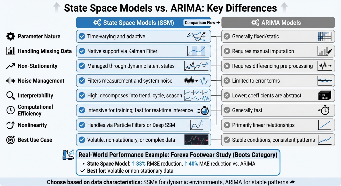
State Space Models vs ARIMA: Feature Comparison for Financial Forecasting
State space models bring flexibility to financial forecasting by allowing parameters to adjust over time, unlike ARIMA models, which rely on fixed parameters. The key difference lies in how these methods respond to change. ARIMA assumes a relatively stable environment, while state space models adapt dynamically to shifting market conditions [3].
This adaptability becomes especially useful when dealing with data challenges. For example, state space models handle missing data seamlessly through the Kalman Filter [19][4], whereas ARIMA requires manual data imputation. Additionally, state space models excel at separating the "true" underlying trend from noisy observations, making them a strong choice for volatile financial datasets prone to market microstructure noise [3].
"The primary benefit of [state space models] is that their parameters can adapt over time." - Quantstart [3]
A practical comparison of these methods was conducted by Portuguese footwear retailer Foreva, which analyzed five product categories using 64 monthly observations between January 2007 and April 2012. In the "Boots" category, the state space model reduced RMSE by 33% and MAE by 40% compared to ARIMA [20]. On the other hand, when applied to quarterly cement production data, ARIMA slightly outperformed with an RMSE of 216 versus 222 for the state space model [21]. These findings highlight that state space models are particularly effective for volatile or non-stationary data, while ARIMA remains a solid option for stable and predictable datasets.
| Feature | State Space Models | ARIMA Models |
|---|---|---|
| Parameter Nature | Time-varying and adaptive [3] | Generally fixed/static |
| Handling Missing Data | Native support via Kalman Filter [19][4] | Requires manual imputation |
| Non-Stationarity | Managed through dynamic latent states [19] | Requires differencing pre-processing |
| Noise Management | Filters measurement and system noise [3][4] | Limited to error terms |
| Interpretability | High; decomposes into trend, cycle, season [19] | Lower; coefficients are abstract |
| Computational Efficiency | Intensive for training; fast for real-time inference [9] | Generally fast |
| Nonlinearity | Handles via Particle Filters or Deep SSM [2][6] | Primarily linear relationships |
| Best Use Case | Volatile, non-stationary, or complex data [3][5] | Stable conditions, consistent patterns [20] |
Since ARIMA and state space models calculate likelihoods differently, traditional metrics like AICc can't directly compare them. Instead, rely on time-series cross-validation or a hold-out test set to determine which model works best for your specific dataset [21][22].
State space models bring practical solutions to some of the most common challenges in financial forecasting. By addressing areas like revenue prediction, cash flow planning, and market regime detection, these models provide a more nuanced and actionable approach.
Revenue forecasting becomes more precise with state space models by breaking down sales data into hidden components like trends, seasonal patterns, and cycles - elements that traditional methods often fail to separate effectively [19][5]. This level of detail helps businesses determine whether a revenue spike is due to actual market growth or simply seasonal demand, which is invaluable for making informed resource allocation decisions.
Cash flow planning benefits from the real-time forecasting capabilities of state space models. Instead of waiting until the end of a financial quarter to reassess cash positions, these models allow weekly updates as new sales data becomes available [10]. They achieve this by rolling forward the current state distribution without requiring a complete re-estimation [5]. For U.S.-based companies managing payroll, inventory, and operating costs in USD, this real-time insight helps avoid costly liquidity issues.
Market regime detection is another powerful application. These models can identify shifts in business phases, such as moving from early-stage customer acquisition to mature scaling, by detecting structural changes in the data [23][5]. This technique, widely used by leading financial institutions, is equally valuable for growth-stage companies aiming to spot changes in marketing ROI or shifts in customer acquisition costs.
These capabilities make state space models an essential tool for addressing complex financial forecasting needs.

Phoenix Strategy Group specializes in integrating state space models into FP&A systems and data engineering workflows, helping growth-stage companies establish reliable and scalable financial forecasting processes. By tailoring these models to specific financial metrics - like subscription revenue, burn rates, or unit economics - Phoenix Strategy Group ensures that forecasts align closely with business realities. This customized approach not only enhances forecasting accuracy but also empowers companies to make better strategic decisions based on actionable insights.
State space models offer a modern solution to the challenges of traditional forecasting by using adaptive parameters that adjust as market conditions change. This makes them particularly useful when historical patterns fail to predict future trends accurately [3]. By leveraging separate state and observation equations, these models can filter out noise, uncover hidden dynamics like latent market volatility or shifts in customer behavior, and naturally produce forecast intervals - giving businesses a clearer picture for decision-making [3][4][5].
The Kalman Filter plays a crucial role by enabling real-time updates to forecasts as new data becomes available, eliminating the need to re-estimate the entire model from scratch [4][5]. These features make state space models a powerful tool for improving financial forecasting.
To make the most of state space models, start with thorough data preparation. Clean your data by removing outliers and consider transformations, such as logarithmic or Box-Cox methods, to stabilize variance before diving into modeling [5]. Opt for advanced estimation techniques like Maximum Likelihood or Bayesian inference rather than relying on basic smoothing methods [4][5]. Above all, treat forecasting as an ongoing process - continuously recalibrate your models with new data, leveraging the recursive nature of state space models [5].
Organizations like Phoenix Strategy Group integrate state space models into FP&A systems and workflows, focusing on critical financial metrics such as subscription revenue, burn rates, and unit economics. Working with experts can help replace generic forecasting tools with tailored systems that empower strategic decision-making.
State space models excel at managing non-stationary financial data by leveraging time-varying state variables that adapt to changes in the data over time. These models incorporate elements like random walks or trends, allowing them to account for shifts in behavior, such as growth patterns or abrupt regime changes, without needing the data to stay stationary.
What makes them particularly useful is their ability to adjust dynamically as fresh data comes in. This adaptability enhances forecasting accuracy, making state space models a powerful tool for financial planning and decision-making in unpredictable or changing markets.
The Kalman Filter is a key component in state space models, offering an efficient method for estimating hidden variables from noisy data. Its recursive process updates predictions in real time, seamlessly integrating new information as it comes in.
This adaptability makes it invaluable for businesses aiming to generate accurate and flexible forecasts, even when faced with uncertainty. By constantly refining its estimates, the Kalman Filter enhances decision-making and planning, particularly in intricate financial scenarios.
State space models stand out in handling volatility due to their ability to adjust parameters dynamically over time. Unlike ARIMA models, which depend on fixed coefficients, state space models leverage the Kalman filter for continuous updates. This approach enables them to respond to shifting trends and real-time noise, making them a better fit for markets that are unpredictable and change rapidly.
By identifying and adapting to evolving patterns, state space models deliver more precise forecasts, equipping businesses with the insights needed to navigate even the most volatile environments effectively.