Published on
December 27, 2025


Electricity price volatility can make or break renewable energy projects. Proper price risk modeling helps investors and developers predict cash flow, secure funding, and make informed decisions. Here’s what you need to know:
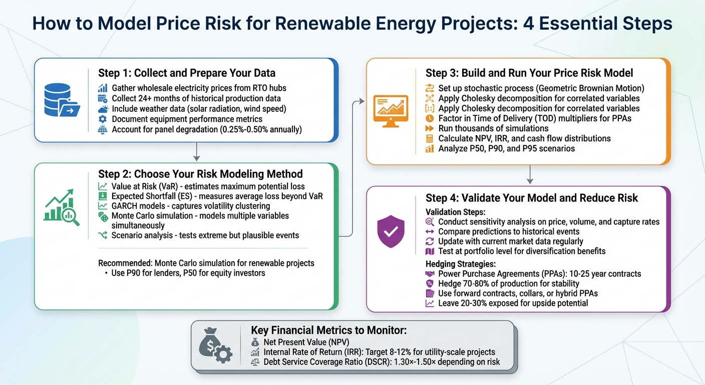
4-Step Process for Modeling Price Risk in Renewable Energy Projects

Price risk refers to the uncertainty in revenue that renewable energy projects face due to fluctuating electricity prices in wholesale markets. Unlike traditional power plants, wind and solar facilities generate electricity only when conditions are favorable. This creates a unique challenge: renewable energy often produces the most power when demand is low or when there is an abundance of supply. As a result, market prices tend to drop precisely when these projects are generating the most electricity.
This dynamic has a major financial impact. A phenomenon called price cannibalization happens when simultaneous production from multiple projects drives down peak prices, creating a gap between the amount of electricity generated and the revenue earned per unit sold [3]. Mark Bolinger from Lawrence Berkeley National Laboratory explains the issue this way:
"For renewable generators like wind and solar projects, resource risk is primarily a quantity risk... Conversely, for gas-fired combined cycle generators, resource risk is primarily a price risk - i.e., the risk that natural gas will cost more than expected" [5].
In simpler terms, renewable energy projects face a double challenge: the weather dictates how much energy they can produce, while market conditions determine the price they earn for that energy. This combination of factors creates significant volatility and highlights the complexity of managing price risk.
Several factors contribute to the price volatility that renewable energy projects experience. One major issue is the widening gap between day-ahead and real-time (DA/RT) prices. This happens when variable renewable generation creates sudden oversupply or undersupply. Another challenge is the daily price fluctuation from peak to trough, as renewable output often peaks during times of lower demand [3]. Additionally, node-to-hub basis risk occurs when transmission congestion prevents projects from receiving the full market hub price [3]. On top of this, weather variability adds another layer of uncertainty - annual production can fall short if wind speeds are lower or cloud cover is heavier than historical averages suggest [5].
Regulatory factors also play a big role in shaping revenue outcomes. Power Purchase Agreements (PPAs), Time-of-Delivery (TOD) price adjustments, capacity payments for maintaining generation availability, and curtailment compensation when grid operators restrict output all affect how much revenue a project can earn [1]. With renewable energy expected to grow from about 25% of total U.S. generation today to approximately 45% by 2030 - and with over two terawatts of solar and wind projects currently in regulatory queues - these challenges are likely to become even more pronounced [3].
Price risk directly impacts key financial metrics like Net Present Value (NPV), Internal Rate of Return (IRR), and Debt Service Coverage Ratio (DSCR). When electricity prices are more volatile than expected, the present value of future cash flows decreases because investors apply higher discount rates to account for the added uncertainty [6]. Even modest market price shortfalls caused by factors like price cannibalization or basis risk can threaten the financial viability of a project.
The IRR is particularly sensitive to price assumptions. In PPA models, the contract price is typically set to achieve a target IRR - often between 8% and 12% for utility-scale projects [1]. If market prices fall short of these projections, merchant plants that sell directly into wholesale markets may see their IRR drop below the cost of capital. Similarly, the DSCR, which measures cash flow available to cover debt obligations, can become strained when revenue volatility increases, raising red flags for lenders [7].
Merchant plants without fixed-price contracts are fully exposed to market fluctuations, meaning they sell electricity at prevailing rates. This can sometimes result in very low or even negative prices during periods of oversupply. Even projects backed by PPAs are not entirely shielded. TOD factors can lower effective prices if generation does not align with high-value delivery times, and curtailment events can significantly reduce revenue during those periods [1]. These financial pressures highlight the need for advanced data analysis and modeling techniques, which will be addressed in the next steps.
To build a reliable price risk model, start by gathering high-quality historical market data and renewable production data. Without accurate and well-organized information, your model may generate unreliable results, leading to poor investment decisions.
Separate your data into two categories: time-independent inputs (e.g., installed capacity, depreciation) and time-dependent inputs (e.g., monthly production profiles, merchant price forecasts) [12]. This approach makes it easier to update your model and evaluate various scenarios, such as comparing P50 and P90 production estimates or analyzing PPA versus merchant pricing structures. With structured data, you can simulate different scenarios seamlessly.
Begin by collecting wholesale electricity prices from the regional transmission organization (RTO) hub where your project operates. The U.S. Energy Information Administration (EIA) provides access to historical data for over two dozen electricity hubs across North America, including markets like PJM West and Mid-Columbia, which offer records dating back to 2001 [9]. Focus on key metrics such as on-peak and daily wholesale spot prices, high/low price ranges, and volumetric weighted-average price indices [8][9].
In addition to electricity prices, gather market liquidity metrics, including daily trade volumes, the number of trades, and participating counterparties [9]. Also, include wholesale natural gas prices from hubs like Henry Hub or Chicago Citygates, as natural gas prices are strongly correlated with electricity prices in many U.S. regions. This data is essential for accurate electricity price modeling, and sources like the Intercontinental Exchange (ICE) offer historical natural gas data going back to March 2014 [9].
Seasonal trends are equally important. For example, in October 2025, wholesale electricity prices across most U.S. regions hit their annual low due to "shoulder" month patterns when mild temperatures reduce energy demand [8]. Incorporating these recurring trends ensures your model accurately reflects revenue fluctuations during low-demand periods.
Finally, complement your market data with detailed production metrics to complete your dataset.
For renewable energy projects, collect high-resolution weather data. For solar projects, this includes mean solar radiation and ambient temperature; for wind projects, gather turbine-height wind speed data. Tools like the National Renewable Energy Laboratory (NREL) System Advisor Model (SAM) provide access to resources like the National Solar Radiation Database (NSRDB) and the WIND Toolkit [7].
Document at least 24 months of historical data for all energy sources to identify performance trends accurately [10]. This should include equipment performance metrics such as nameplate capacity, efficiency ratings, operating hours, and historical production rates [10]. Use utility revenue meters as your primary source for historical consumption and delivery data [10].
Adjust raw resource data to reflect technology conversion efficiencies [11]. For example, monocrystalline PV cells differ from polycrystalline cells in terms of efficiency, which directly impacts revenue projections [11]. Perform integrity checks to ensure your data is accurate - such as confirming that monthly profiles sum to 100% - and use visual cues to differentiate raw data, calculations, and constants [12]. Don’t forget to account for panel degradation rates, which typically range from 0.25% to 0.50% per year, leading to an 8% to 15% reduction in output over a 30-year project lifespan [12].
With your data prepared, the next step is selecting a risk modeling method that aligns with your project's complexity and revenue structure. The method you choose will shape how well you capture price fluctuations and production uncertainties in your financial forecasts.
To assess price risk, you can use methods like Value at Risk (VaR), Expected Shortfall (ES), GARCH models, and scenario analysis.
For a more comprehensive approach, consider incorporating Monte Carlo simulation.
Monte Carlo simulation is especially well-suited for renewable energy projects because it can model multiple unpredictable variables at once, such as weather-dependent production, future cash flows, and fluctuating market prices [12]. Unlike sensitivity analysis, which examines one variable at a time, Monte Carlo handles overlapping and complex market conditions more effectively [2][7].
This method assigns statistical distributions to input variables, allowing you to calculate the probability that annual outputs will exceed certain thresholds. The results are expressed as P-values (P50, P75, P90), which correspond to different levels of risk [7]. For instance, P90 represents a conservative estimate with a 90% probability of being exceeded, while P50 reflects the median expected outcome [12].
A case study from April 2021 highlights Monte Carlo’s advantages. Moody’s RMS conducted a risk assessment for a 17-square-mile wind farm on the Texas coast with 76 turbines. By using RMS North Atlantic Hurricane Models and replacing a single-point geocoding approach with a detailed model of each turbine's location, they discovered that average annual loss (AAL) estimates varied by as much as 30% depending on turbine placement [13]. This example underscores Monte Carlo's ability to account for spatial variability and multiple risk factors, providing more reliable results than simpler methods.
When applying Monte Carlo simulation, use P90 values for lender-focused scenarios and P50 values for equity-based cases [12]. This dual approach helps meet both financing needs and strategic decision-making goals.
Now that you’ve selected your modeling method, it’s time to build and execute your price risk model. This step is crucial for understanding how price fluctuations impact key financial metrics. Essentially, it transforms your prepared data into actionable risk insights.
Start by implementing a random (stochastic) process to simulate price scenarios. A common approach is Geometric Brownian Motion (GBM), which works well for modeling price movements that behave like stocks. Using GBM involves estimating three main variables - drift (μ), volatility (σ), and the initial price (S₀) - based on historical market data [15]. If prices tend to revert to a long-term average, consider using mean-reverting models like the Ornstein-Uhlenbeck (O-U) or Cox-Ingersoll-Ross (CIR) models [15][16].
For projects with multiple interconnected variables - such as energy prices and production volumes - use Cholesky decomposition to introduce correlation between variables from independent random draws [15]. If you’re working with Power Purchase Agreements (PPAs), don’t forget to factor in Time of Delivery (TOD) multipliers. These adjust the base PPA price based on the time of day or season, capturing the impact of generation timing on renewable energy revenue [1].
To handle large-scale computations efficiently, use vectorized coding in tools like R or Python to simulate multiple price paths at once. Boost the accuracy of your simulations by applying techniques like Antithetic Variables or Control Variates [15].
Once your model is set up, you’re ready to run simulations and analyze the outcomes.
Run thousands of simulations to generate a range of possible outcomes. For GBM, the price at each future time step is calculated as:
S(t+h) = S(t) exp[(μ - 0.5σ²)h + σε√h]
Here, ε represents a random draw from a standard normal distribution [15]. After completing the simulations, calculate the Value at Risk (VaR) by identifying the loss threshold at your chosen confidence level - typically 95% or 99% [15].
Use the simulation results to analyze distributions for key financial metrics like Net Present Value (NPV), Internal Rate of Return (IRR), and cash flow projections [1][7]. For renewable energy projects, you can approach this in two ways: either set an IRR target and determine the required PPA price, or specify a PPA price and calculate the resulting IRR [1]. Dive deeper into cash flow outputs to identify potential shortfalls in revenue that could affect operating costs or debt service. Including additional revenue sources - like capacity payments or curtailment compensation - provides a more comprehensive view of potential returns [1].
The results will help you understand not only the median outcome (P50) but also more conservative scenarios like P90 or P95. These downside scenarios are especially critical for determining debt sizing and managing financial risk effectively [5].
Once you've completed your simulations, the next crucial step is to validate your model. This means checking it against historical data and sensitivity tests, then using those insights to minimize risks. It’s all about transforming your hard-earned analysis into actionable risk management strategies.
Begin with a sensitivity analysis to see how changes in critical factors - like price, volume, or capture rates - impact your financial outcomes. For example, a 2022 analysis of a 1,154,184 MWh portfolio revealed that a 10% drop in price slashed revenue by $7,423,186, while a 10% dip in volume resulted in a $12,045,500 loss [17].
Next, compare your model's predictions to real-world historical events to ensure it behaves realistically. For instance, check if it would have captured the pricing surge seen in Q4 2021. Pay close attention to P90 results, which represent a conservative forecast where there's a 90% likelihood of meeting or exceeding expectations. In one case, P90 simulations showed unhedged revenue dropping from $77.9 million to $65.2 million [17].
Keep your model up to date by incorporating current market data, regulatory changes, and production figures. As Maritina Kanellakopoulou from Pexapark puts it:
"Inertia is only good for the electricity grid, not for business plans" [17].
If you're overseeing multiple projects, validate your model at the portfolio level. This approach can help you quantify diversification benefits, as risks in one region or technology might offset those in another [17].
Once your model checks out, the next step is to focus on reducing risk through hedging strategies.
Armed with a validated model, you can use hedging to stabilize revenue streams. Power Purchase Agreements (PPAs) remain a popular choice, offering long-term price stability through contracts lasting 10–25 years. Depending on your needs, you can explore different types of PPAs:
Many investors hedge 70%–80% of their production to secure predictable revenues for debt financing, leaving 20%–30% exposed to potential price gains [17]. As C. Onur Aydin from Brattle explains:
"Due to the uncertain volume of production from a weather-dependent resource, it will be impossible to fully or perfectly hedge, especially over very short horizons. However, the average output from a renewable resource over horizons of a year or longer is more predictable and can be hedged" [19].
For mid-term hedging, standard forward contracts work well. To manage exposure during volatile market swings, consider collars that set price floors and caps [19]. In regions where gas and electricity prices are closely linked, gas forwards can act as a proxy hedge - just be sure to account for basis risk from delivery location differences [19]. Lastly, monitor unrealized profit and loss by counterparty to identify significant discrepancies that may require renegotiation [17].
Once your price risk model is validated, its real power comes into play when you integrate it into financial decision-making. By adjusting project valuations to account for uncertainty and presenting risk insights clearly, you can capture market variability and guide strategic choices. Below, we explore how to refine financial models and effectively communicate risk insights.
Standard Discounted Cash Flow (DCF) models often rely on a single scenario, which doesn't account for the uncertainty surrounding renewable energy prices and production. Instead, consider using probabilistic forecasting with weighted outcomes, building on the simulation results from earlier steps [24].
Start by aligning your discount rate with the project's risk profile. For instance, utility-scale solar PV supported by a Power Purchase Agreement (PPA) might require an after-tax equity return of 7.75%, whereas quasi-merchant natural gas projects, with higher revenue uncertainty, could demand around 10.0% [23]. For renewable energy technologies, the Weighted Average Cost of Capital (WACC) typically ranges from 4.2% to 5.3% in R&D-focused cases [23].
It's also crucial to differentiate between fixed-price revenue streams (like PPAs or Feed-in Tariffs) and merchant revenue, which is subject to market fluctuations. Merchant projects often carry a premium of 100 basis points or more on the cost of equity [23]. When projecting cash flows, incorporate energy yield probability values - equity investors often prefer P50, while debt investors lean toward P75 or P90 to ensure debt repayment under less favorable production scenarios [21][22].
Price volatility plays a significant role in determining the Debt Service Coverage Ratio (DSCR). For wind projects, higher price risk might push lenders to require a DSCR of 1.40× to 1.50×, compared to about 1.30× for solar PV. This can reduce leverage and impact the levered Internal Rate of Return (IRR) [22][23].
Simulations can help you create ranges of outcomes with associated probabilities. As Richard Morris from Harvard Business Review's Advisory Council notes:
"Probably the single, most effective change that can be made is to incorporate probability weighting into FP&A forecasts to better capture the uncertainty and variability inherent in predicting future events" [24].
To gain more dynamic insights, connect pricing and production efficiency with macroeconomic factors, especially during the construction phase when risks are higher [23].
Once your cash flow projections are refined, the next challenge is presenting these risk-adjusted valuations in a way that stakeholders can easily understand.
Turning complex risk models into clear and actionable insights requires a strategic approach to presentation. A centralized dashboard can provide decision-makers with a quick snapshot of critical investment metrics and key performance indicators [12]. This builds on the simulation results and DCF adjustments already discussed. As Lukas Duldinger, CFA, puts it:
"The investment dashboard is the output heart of the model. It gives decision-makers an instant overview of the essential investment metrics any decision-maker should consider before investing" [12].
Tailor your presentation to the audience. For instance, show Net Present Value (NPV) adjustments for investor targets or relative project worth for developers. Include energy yield and revenue forecasts using P50, P75, and P90 values - lenders typically prioritize P90 for debt sizing, while equity investors focus on P50 [12].
Use scenario and sensitivity analyses to illustrate valuation changes under varying market conditions. For example, compare a "Fully Merchant" scenario with one based on a "10-year PPA", or adjust merchant price forecast curves between central and low cases. Adding interactive elements, like drop-down menus in financial models, allows stakeholders to see real-time updates when switching between contract scenarios [12].
Transparency is essential for building trust. Clearly document and justify key variables, such as a 2.5% inflation rate based on historical U.S. consumer price index data, discount rates, or equipment degradation assumptions (e.g., high-quality solar panels typically degrade by 0.25% to 0.50% annually, leading to an 8.0% to 15.0% output reduction over 30 years) [12][25]. Use visual aids like graphs and tables to simplify complex models, and standardize elements - such as marking adjustable input cells in light blue - to make it clear what variables are being tested. Finally, update models regularly with fresh market data and compare past forecasts to actual outcomes. This helps identify biases and refine future projections [6].
Modeling price risk in renewable energy projects requires accurate data, effective modeling techniques, and strategies to manage risks. As Mark Bolinger of Lawrence Berkeley National Laboratory explains:
"For renewable generators like wind and solar projects, resource risk is primarily a quantity risk - i.e., the risk that annual energy production will be less than expected due to a weaker-than-expected wind or solar resource" [5].
Recognizing the difference between quantity risk (variability in production) and price risk (market price changes) is essential for creating models that mirror actual conditions.
It all begins with data. Tools like NREL's SAM provide a framework for evaluating renewable projects, but as noted in the SAM documentation:
"It is your responsibility as an analyst to review and modify all of the input data as appropriate for each analysis" [7].
This means analysts must go beyond default settings, verifying and customizing inputs to suit each specific project. A solid data foundation allows for the application of advanced techniques like Monte Carlo simulations, which transform single-point estimates into ranges of potential outcomes. By shifting from P50 (expected) to P90 (conservative) scenarios, these simulations offer lenders and equity investors the assurance they need to support a project.
The final steps in your strategy involve validation and hedging. Regularly testing models through sensitivity analysis, updating them with current market data, and incorporating hedging tools like Power Purchase Agreements (which often span 10 to 25 years [2]) can help safeguard against unfavorable scenarios. Additionally, setting up reserve accounts for major maintenance and using P90 estimates for debt sizing can ensure your project remains resilient against both operational and market uncertainties.
With these elements in place, your renewable energy project is better equipped to handle the complexities of price risk.
Price cannibalization happens when an increase in energy production pushes market prices down, which can cut into revenue. To tackle this challenge, renewable energy projects can adopt a mix of hedging strategies and financial modeling:
By blending these strategies with proactive scenario analysis, developers can prepare for and mitigate price cannibalization risks. Phoenix Strategy Group specializes in crafting hedging solutions, building financial models, and providing contract advice to help keep your project financially secure.
Power Purchase Agreements (PPAs) are essential tools for managing price risks in the energy sector. They offer price stability by setting a fixed rate for electricity over the duration of the contract. This shields both energy producers and investors from unpredictable market price swings.
With a steady and predictable revenue stream, PPAs help reduce financial uncertainty. This makes it easier for energy projects to secure funding and plan operations over the long term. This is particularly important for renewable energy projects, where electricity prices can fluctuate due to factors like changing supply and demand or shifts in regulations.
Monte Carlo simulation is a popular tool for analyzing the uncertainty and volatility of renewable energy prices. By simulating thousands of possible price scenarios, it provides a probabilistic view of risks, giving project developers and investors the insights they need to make smarter decisions.
What sets Monte Carlo simulation apart from traditional methods is its ability to account for the unpredictable nature of renewable energy markets. Factors like shifting demand, weather variability, and policy changes can heavily influence outcomes. This method minimizes bias and offers a clearer understanding of potential scenarios, making it a go-to strategy for managing financial risks in renewable energy projects.