Published on
February 12, 2026


STL decomposition is a method to break down financial data into three parts: trend, seasonality, and residuals. This approach helps businesses identify true growth patterns, separate recurring seasonal effects, and account for unexpected anomalies in their data.
Key Takeaways:
By using STL, you can:
STL is flexible, handles outliers effectively, and is customizable for various business needs. Tools like Python's statsmodels make it easy to apply STL for financial forecasting and decision-making.
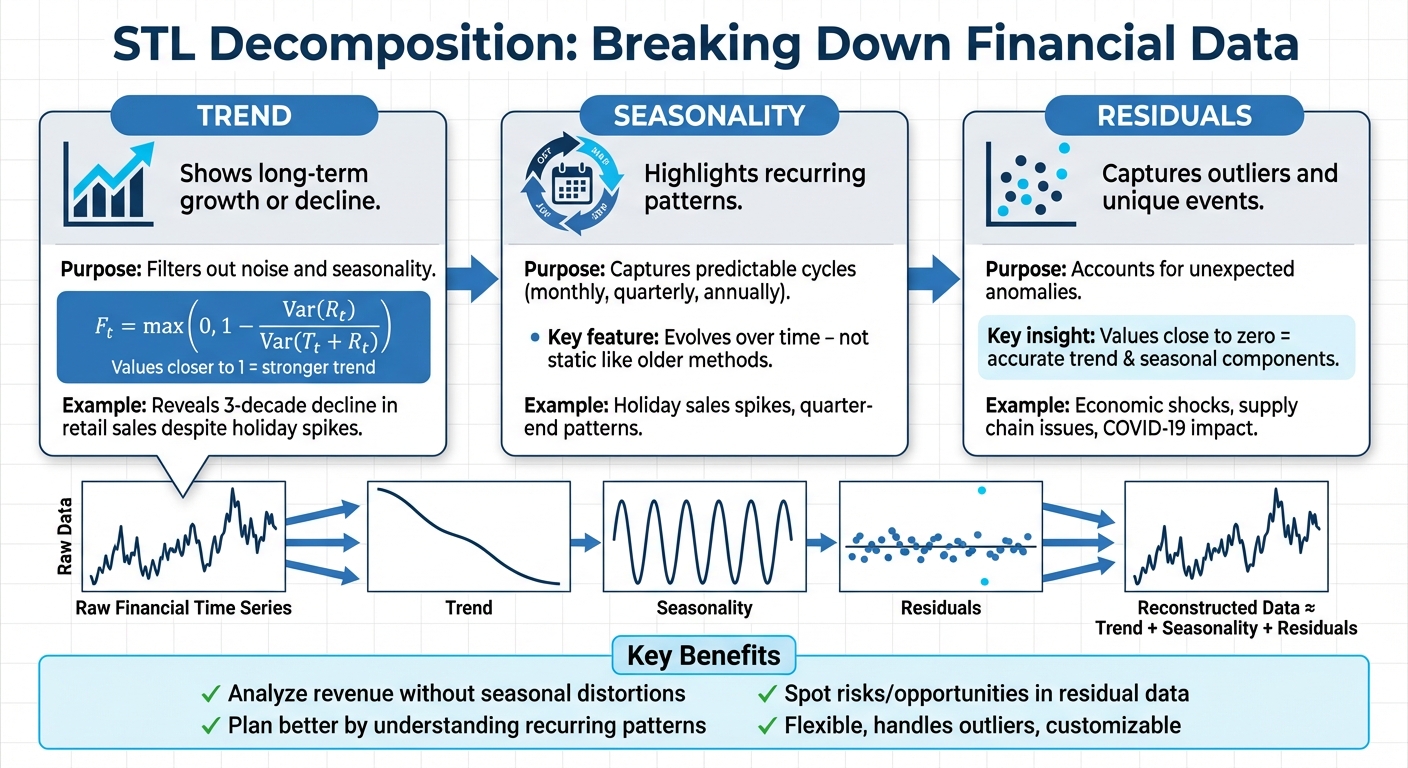
STL Decomposition Three Components Explained: Trend, Seasonality, and Residuals
STL breaks down financial data into three core components: Trend (long-term movement), Seasonal (recurring patterns), and Residual (unexpected deviations that don't align with the trend or seasonality).
At its heart, STL uses LOESS (Locally Estimated Scatterplot Smoothing) to handle complex, non-linear growth patterns with precision [4][1]. By adjusting the window settings, you can control how smooth or responsive these components are, allowing STL to capture everything from sharp fluctuations to steady trends [4]. This adaptability makes STL a powerful tool for detailed financial management and analysis.
The trend component highlights the long-term direction in your data, filtering out seasonal effects and random noise [4][6]. Essentially, it gives you a clear picture of where your metrics are heading over time.
To measure the strength of the trend, STL uses the formula:
Fₜ = max(0, 1 - Var(Rₜ) / Var(Tₜ + Rₜ)),
where values closer to 1 indicate a stronger, more dominant trend [5]. Beyond this, analyzing the linearity and curvature of the trend can reveal whether growth is steady, accelerating, or slowing down [5].
For example, in a study of U.S. department store retail sales from January 1992 to March 2025, the trend component uncovered a gradual decline spanning three decades. Despite significant holiday spikes in the raw data, STL identified the underlying downward trajectory. Even during the COVID-19 shock in early 2020, the trend remained stable, correctly showing that the sales drop was temporary rather than a lasting change [2].
"The smoothness of the trend-cycle can also be controlled by the user... It can be robust to outliers so that occasional unusual observations will not affect the estimates of the trend-cycle."
- R. J. Hyndman and G. Athanasopoulos, Forecasting: Principles and Practice [4]
The seasonal component captures predictable, recurring patterns in your data - whether they occur monthly, quarterly, or annually [3]. These patterns often reflect things like holiday sales, quarter-end spikes, or other regular fluctuations.
Unlike older techniques that assume static seasonal patterns, STL allows the seasonal component to evolve over time [4][2]. This flexibility is particularly useful when seasonal peaks shift or change in intensity. By adjusting the seasonal window, you can fine-tune your analysis - using smaller windows for rapidly changing patterns or setting it to "periodic" for consistent cycles.
Once isolated, the seasonal component serves multiple purposes. You can subtract it from raw data to "deseasonalize" the numbers, helping you determine if a revenue dip is part of normal seasonal variation or something more concerning [6]. Additionally, you can project the seasonal pattern forward and combine it with the trend forecast for better future predictions [1].
The residual component accounts for everything that the trend and seasonal components don't explain. This includes one-time events, outliers, and irregular variations [2]. Think of this as the "catch-all" for unexpected disruptions, such as supply chain issues, legal events, or economic shocks.
"Values close to zero [in the remainder] indicate that the seasonal and trend components are accurate in describing the time series."
Running STL in robust mode ensures that outliers are placed into the residual component rather than distorting the trend or seasonal patterns [4][2]. This way, unusual events don't skew your understanding of long-term performance, helping you make more reliable conclusions about your financial data.
STL addresses common hurdles in financial analysis, such as shifting seasonal trends, market volatility, and diverse analytical requirements. Unlike older methods that assume static seasonal patterns, STL adjusts to dynamic market behaviors and consumer trends [2][4]. Its ability to separately control components like trend smoothness and seasonal changes makes it versatile, whether you're analyzing daily cash flows or quarterly performance metrics [4]. Below, we explore how STL's flexibility, resilience to outliers, and customizable parameters make it a valuable tool for financial data analysis.
STL uses LOESS smoothing by analyzing subseries (for instance, all January data across several years) to detect evolving seasonal trends rather than assuming fixed cycles [2][4][6]. This adaptability is crucial for identifying financial outliers. For example, in a study of U.S. retail sales from 1992 to 2025, STL effectively tracked changing holiday shopping patterns while isolating the January 2020 COVID-19 shock as a one-time anomaly [2]. Analysts can fine-tune this adaptability using the seasonal window parameter - smaller values make the model more responsive to rapid changes, while larger values create smoother seasonal trends [4][1].
Financial data often includes unexpected spikes caused by events like large payments, unforeseen expenses, or economic disruptions. These anomalies can distort traditional analyses. STL's robust mode uses adaptive weighting to downplay extreme values [1]. This ensures that sudden anomalies appear in the residual component, leaving trends and seasonal estimates unaffected [4][6].
"Using robust estimation allows the model to tolerate larger errors."
- Statsmodels Documentation [1]
During the 2008 financial crisis, robust STL successfully isolated a significant drop in EU electrical equipment production, preserving the underlying trend [1]. For growing businesses, this means that one unusual period won't throw off long-term growth projections [4][3]. Additionally, examining residual variance can highlight hidden volatility, helping analysts identify potential risks or anomalies early [3][6]. This feature not only clarifies trends but also serves as an early warning system for financial instability.
STL's parameters are highly customizable, making it suitable for various analytical objectives, from long-term forecasting to spotting irregularities. The trend and seasonal window settings, in particular, allow analysts to balance smoothness with responsiveness [4].
| Parameter | Function | When to Adjust |
|---|---|---|
| Trend Window | Controls the smoothness of the trend | Use smaller values for rapid changes; larger for stable trends [4] |
| Seasonal Window | Adjusts how seasonal patterns evolve | Use smaller values for fast-changing patterns; larger for consistent cycles [4][1] |
| Robust Setting | Reduces the impact of outliers | Always enable for volatile financial data [1] |
For example, when analyzing U.S. retail employment, the default trend window was too rigid, allowing the 2008 economic crisis to influence the residual component. By shortening the trend window, analysts captured rapid economic shifts more accurately [4]. These adjustable settings enable financial professionals to tailor STL to specific business needs, ensuring the model reflects the unique dynamics of their data instead of forcing it into a generic framework.
Now that we’ve covered the basics of STL decomposition, let’s dive into how you can use it to analyze financial data in Python. With just a few lines of code, you can break down your data into trend, seasonal, and residual components using the statsmodels.tsa.seasonal.STL library. This tool leverages LOESS smoothing to give you a clear picture of your dataset's underlying patterns [1].
To get started, make sure your financial data is well-structured. Ideally, it should be in a Pandas Series or DataFrame format, with a datetime index and a defined frequency (like 'MS' for month-start data). Selecting the right parameters is crucial here - done correctly, it lets you spot anomalies without distorting the overall trend. Below, we’ll walk through the process step by step.
Implementing STL decomposition in Python is straightforward. Here’s how you can do it:
.asfreq('MS'). If your data lacks a natural frequency, you can specify one (e.g., period=12 for monthly data).
stl = STL(data['revenue'], seasonal=13, robust=True)
result = stl.fit()
.plot() method to generate a chart showing the original data, trend, seasonal, and residual components side by side.
This approach makes it easy to see how your financial data behaves over time.
Once your data is ready, the next step is fine-tuning the STL parameters to suit your specific dataset. There are three key parameters to consider:
seasonal=13.robust=True helps handle outliers, such as one-off large contracts or unexpected expenses, ensuring they don’t distort the trend.All window sizes must be odd integers, and experimenting with these values can help refine your analysis.
Once you’ve run the decomposition, it’s time to dig into the results. Each component provides unique insights:
If you notice patterns in the residuals or see the trend mimicking seasonality, revisit your parameter settings to fine-tune the decomposition. For datasets with multiplicative growth (where changes are proportional rather than absolute), applying a natural logarithm transformation before decomposition - and back-transforming afterward - can make the results easier to interpret in dollar terms.
These insights can guide critical decisions, from resource planning to forecasting and managing risks. By carefully analyzing each component, you’ll uncover trends and anomalies that might otherwise go unnoticed, giving you a clearer view of your financial performance.
STL decomposition offers a powerful way to break down complex financial data into trends, seasonality, and residuals, making it easier for growth-stage businesses to navigate challenges like seasonal shifts, unexpected events, and rapid scaling. By separating these components, businesses can make more informed financial decisions.
For businesses experiencing growth, understanding whether a December revenue surge is part of a long-term trend or simply holiday seasonality is crucial. STL makes it possible to separate these influences, helping you forecast more accurately. By isolating the trend, you can assess real growth, while the seasonal component helps you plan for cash flow, staffing, and inventory needs [8].
If your business is experiencing multiplicative growth, consider applying a log transformation to revenue before using STL [4]. Tools like STLForecast allow you to remove seasonality, apply forecasting models like ARIMA to the adjusted trend, and then reintroduce the seasonal pattern for more precise predictions [1]. These refined forecasts help you anticipate risks and make proactive decisions.
STL decomposition doesn't just support forecasting - it also enhances your ability to identify risks and opportunities. The residual component, which captures fluctuations not explained by trends or seasonality, acts as an early warning system. Large residual spikes can signal potential risks or highlight new opportunities that deserve attention [3].
"STL... can be robust to outliers (i.e., the user can specify a robust decomposition), so that occasional unusual observations will not affect the estimates of the trend-cycle and seasonal components. They will, however, affect the remainder component."
- Forecasting: Principles and Practice (3rd ed) [4]
By using robust fitting, you can ensure outliers are confined to the residuals, keeping your trend and seasonal estimates accurate [4][1]. Regularly auditing the residuals can help you catch operational issues or uncover untapped market opportunities early on [3].
STL decomposition also simplifies the analysis of seasonally adjusted KPIs, enabling more accurate comparisons across different periods [7]. This is especially important when presenting your business's performance to investors or board members.
For example, an analysis of U.S. Department Store Retail Sales data from January 1992 to March 2025 showed how STL correctly identified the January–February 2020 sales drop as a one-time anomaly caused by COVID-19, rather than a permanent shift in the trend. A simple moving average might have misinterpreted this as a structural change [2]. For businesses scaling or entering new markets, STL's adaptive seasonal component offers a more accurate approach than traditional decomposition methods [2][4].
When tracking KPIs, keep an eye on residuals. Values close to zero suggest that your trend and seasonal components are accurately reflecting business performance. Larger residuals, however, may indicate noise or anomalies that require further investigation [6].

In today’s fast-moving markets, traditional financial models often fail to keep up. Phoenix Strategy Group offers a modern alternative by using AI-powered FP&A systems and time-series forecasting. By applying data-driven STL insights, they help businesses pinpoint real growth trends, manage seasonal fluctuations, and make smarter, data-informed decisions. Their approach takes STL’s capabilities and transforms them into actionable, real-time insights that guide strategic decision-making.
STL decomposition plays a key role in uncovering critical growth patterns, and Phoenix Strategy Group takes this a step further by enhancing forecasting methods. Through their Fractional CFO and FP&A services, they implement advanced tools like Prophet models and State Space Models (Kalman Filter). These tools are designed to handle the noisy, non-stationary financial data that growing businesses often encounter. This makes it possible to filter out seasonal variations and one-off anomalies, leaving only the core growth signals. Additionally, their Data Engineering services provide the infrastructure necessary to process and break down financial data into trend, seasonal, and residual components - an essential step for STL decomposition to function effectively.
"Startup financial models are the mission control of your startup." - Phoenix Strategy Group [9]
A key part of their methodology is ensuring that financial models stay reliable, even in volatile markets. By automating the analysis of trends and seasonality through integrated financial systems, they create workflows that make decomposition seamless. Their "Systems First" approach helps founders shift from hands-on growth management to scalable operations, supported by customized KPIs and real-time financial insights.
For companies ready to embrace advanced techniques like STL decomposition, Phoenix Strategy Group offers the tools, expertise, and data infrastructure needed to turn complex time-series data into clear, actionable insights. Their focus on unit economics - such as LTV, CAC, and contribution margin - and rolling forecasts ensures that the insights gained from decomposition translate into practical financial strategies. This approach enables businesses to achieve sustainable growth while maintaining a clear view of their financial health.
STL decomposition has transformed how financial data is analyzed by breaking it down into three key components: trend, seasonality, and residual noise. By separating these elements, it becomes easier to identify real growth trends while filtering out short-term fluctuations. This prevents overreacting to market volatility and helps focus on long-term strategies [3].
Unlike older techniques that rely on fixed seasonal assumptions, STL adjusts to changes as businesses and markets evolve. This flexibility is crucial since market conditions are rarely static [2]. Additionally, STL’s robust fitting feature ensures that extreme outliers - like those seen during economic crises - don’t skew the trend line, maintaining accuracy when it matters most [1].
STL’s design also supports better forecasting and risk management. By isolating seasonal patterns and minimizing noise, forecasts become more reliable. Meanwhile, the residual component can act as an early warning system for potential financial risks [3][6]. Historical studies have demonstrated STL’s strength in tracking shifting seasonal trends over time [2].
Although it was introduced back in 1990, STL remains a valuable tool as businesses increasingly lean on adaptable modeling techniques [3]. Learning to use STL effectively can improve data clarity, ensuring smarter resource allocation and more informed strategic decisions.
When choosing seasonal and trend window sizes for STL decomposition, keep your data's periodicity and the level of smoothness you want in mind:
It's a good idea to experiment with these values to find the best fit for your dataset.
When working with time series data that includes anomalies, outliers, or abrupt shifts in trends or seasonal patterns, robust STL is a great option. Its ability to handle irregularities ensures that trends and seasonal components remain accurate without being distorted by unexpected deviations. This makes it particularly useful for challenging datasets, such as financial data, where unpredictability is common.
However, if your dataset is clean and exhibits stable trends and seasonality, robust STL might not be the best choice. Simpler methods can often do the job effectively in such cases, and using robust STL could unnecessarily complicate the analysis or even risk overfitting minor noise in the data.
Log-transforming revenue isn’t a requirement for STL decomposition. However, it can be helpful if you’re aiming for a multiplicative decomposition. To achieve this, simply take the logarithm of your data before performing the decomposition. Once the process is complete, you can back-transform the results to make them easier to interpret.