Probabilistic Sensitivity in Renewable Finance Models

If you only use base, upside, and downside cases, you’re missing the main question: what are the odds the project misses DSCR or equity return targets?

I’d sum the article up like this: deterministic cases show a few fixed answers, while probabilistic methods show a range of outcomes and the chance of each one. In renewable finance, that matters because inputs like energy yield, merchant prices, curtailment, O&M, degradation, and debt terms can move together, and small shifts can change lender and sponsor decisions.

Here’s the short version:

• Monte Carlo runs thousands of simulations instead of just 3 cases
• It helps estimate the odds of missing DSCR, IRR, NPV, or LCOE targets
• It can reflect linked inputs, like higher generation lining up with lower power prices
• FAST, EFAST, and Sobol do a different job: they show which inputs drive output variance
• That ranking can shape debt sizing, DSRA levels, hedge focus, EPC terms, and contingency budgets
• The article points to examples like:
  • 100,000 simulations in a 2024 hybrid wind/solar study
  • failure events every 250 to 1,000 days cutting target-hit odds by 3%
  • a 2026 rooftop PV study where electricity price escalation had sensitivity scores of 0.47 for NPV and 0.919 for payback
  • a case where a 10% CAPEX overrun hurt DSCR more than a 5% PPA price cut

A simple way I’d think about it:

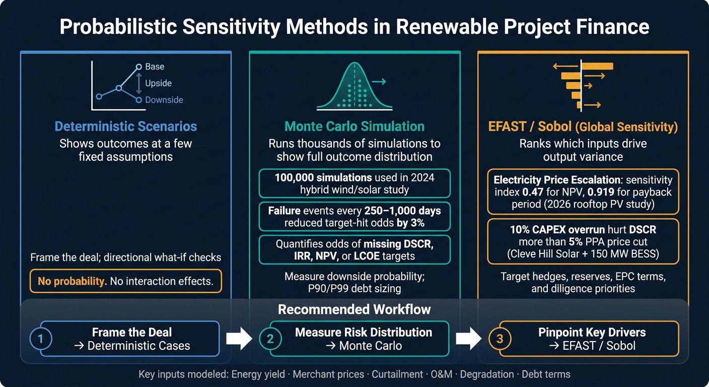
My takeaway: use all three in order. Start with fixed cases to frame the deal. Then use Monte Carlo to test downside odds. After that, use global sensitivity analysis to see where diligence, contract terms, and downside protection should be focused.

That’s the core message of the article in plain English.

Monte Carlo simulation: converting uncertain inputs into outcome distributions

How Monte Carlo works in a renewable cash flow model

In a Monte Carlo model, you don't plug in one fixed number for each assumption. You assign a probability distribution to each uncertain input instead: energy yield, capex, opex, merchant power prices, curtailment, degradation, and interest rates. Then the model runs thousands of cash flow simulations based on those distributions. The output is a range of IRR, DSCR, and NPV results.

Why does that matter? Because the model is only as good as the way those distributions are set up and run.

For lenders and sponsors, the biggest inputs are usually energy yield, availability, and price. A common setup uses a distribution centered on the P50 estimate - the value with a 50% probability of exceedance ^[6][7]. P75 and P99 fall below P50 based on the modeled spread. That gap matters a lot for debt sizing.

Solar degradation, curtailment, and availability make things more nuanced. Many models assume a flat 95% plant availability. In practice, outages and curtailment can drag availability down to about 91% by year 10 ^[3]. Degradation is often modeled at –0.4% per year ^[3]. Monte Carlo helps map those long-term factors across thousands of simulated paths. It can also pick up non-linear effects, like temperature changes hitting solar output or high wind speeds cutting turbine output ^[4].

A 2024 hybrid solar/wind case study using 100,000 simulations showed that added wind improved target-matching odds, and that failure events occurring every 250 to 1,000 days reduced the probability of meeting energy targets by 3% ^[4].

What Monte Carlo adds beyond simple scenario analysis

For debt sizing, Monte Carlo links outcome distributions straight to covenant risk. Lenders calculate Cash Flow Available for Debt Service under both P50 and P99 cases, and the lower CFADS case becomes the binding constraint ^[6].

A three-case model shows what happens if assumptions land at three fixed points. Monte Carlo does more than that. It shows how often a project may miss its DSCR covenant or how often equity IRR may fall below the hurdle rate across the full mix of possible input combinations.

One modeling detail matters here: CFADS should be recalculated in every iteration because revenue-linked costs and taxes move with simulated yield and prices ^[6].

Once that outcome range is visible, the next job is figuring out which inputs are doing most of the work.

sbb-itb-e766981

Completed Monte Carlo Analysis in Project Finance Model

Global sensitivity analysis: FAST, EFAST, and Sobol methods explained

Once Monte Carlo shows the range of possible outcomes, GSA helps answer a different question: which inputs are doing most of the work?

What variance-based methods measure

Variance-based methods split the total variance of a model output into parts linked to each input. A first-order sensitivity index shows an input’s direct share of output variance. A total-effect index goes further and includes that input’s interaction effects with other variables.

A 2026 rooftop PV study found Electricity Price Escalation Rate was the top driver of NPV and payback period, with sensitivity indices of 0.47 and 0.919 respectively ^[1]. For a project finance team, that kind of ranking is hard to ignore. It shows where diligence, contract terms, and risk controls deserve the most attention.

How EFAST and Sobol methods differ from Monte Carlo alone

EFAST - Extended Fourier Amplitude Sensitivity Test - uses Fourier-based sampling to estimate sensitivity indices with good efficiency, without materially increasing simulation runs ^[1][2]. Sobol methods use a different variance-decomposition approach. In both cases, the output is a ranked set of sensitivity indices for each input.

That’s the key difference. Monte Carlo shows the distribution. EFAST and Sobol show what drives it. And that can change the conversation. If one variable dominates NPV or DSCR variance, the team may lean harder on hedges, bigger reserves, or tighter contract terms, such as fixed-price EPC contracts or a more conservative debt service reserve account.

Local versus global sensitivity methods: when to use each

Spreadsheet-style one-at-a-time (OAT) sensitivity, the kind behind most tornado charts, changes one variable while holding the rest fixed. It’s fast, familiar, and easy to explain in a meeting. But it leaves out two things that matter a lot in renewable finance models: nonlinearity and interaction effects.

Here’s the problem in plain English: project variables don’t move in isolation. When two inputs shift together, their combined effect on DSCR may look very different from what one-at-a-time testing suggests. That’s where local methods can give a neat answer to a messy problem.

Global methods like EFAST and Sobol vary all inputs at the same time across their full ranges. That lets them capture the nonlinear behavior and interaction effects that local tests can miss. So the right method depends on the decision in front of you.

Where probabilistic sensitivity fits in project finance decisions

These methods feed straight into lending and investment calls. Once a model shows the range of outcomes and the variables that move the numbers most, the focus shifts fast: How do lenders and sponsors use that view in an actual deal?

Debt sizing, covenants, and downside protection

In project finance, lenders usually size debt with a two-test approach. They test debt capacity under both P50 and P99 production cases, then use the lower result as the debt cap ^[5].

Probabilistic CFADS analysis helps turn covenant risk into something more concrete. It shows how likely cash shortfalls are under different production and pricing paths. That, in turn, shapes debt sculpting, covenant thresholds, and DSRA sizing ^[5].

A good example comes from the Cleve Hill Solar + 150 MW BESS project. There, a 10% CAPEX overrun reduced DSCR more than a 5% PPA price cut, which pushed lenders toward a fixed-price EPC contract ^[3].

Equity returns, valuation, and risk-adjusted investment cases

For sponsors, the same analysis serves a different job. The focus moves from credit protection to valuation and return planning.

Sponsors use P50 estimates to build base-case IRR and project valuation ^[5][7]. Monte Carlo outputs then show the downside tail in plain terms, including the likelihood of hitting hurdle rates. Global sensitivity methods help sort the main drivers of IRR and NPV, which can steer contract talks, contingency budgets, and hedging priorities ^[3][8].

How advisory teams can apply these methods in practice

In practice, the way you present the output matters almost as much as the output itself. Simulation detail should stay in the appendix. For the board or investment committee memo, it's better to lead with tornado charts and clear probability statements ^[3].

Phoenix Strategy Group can turn these outputs into lender-ready forecasts and investment committee materials.

Conclusion: key findings and takeaways for decision-makers

Deterministic scenarios help set the frame for a deal. But on their own, they don't show probability or how variables interact. Monte Carlo fills that gap. It turns uncertain inputs into a distribution, so teams can measure the odds of hitting financial targets across the full spread of NPV, IRR, or LCOE outcomes.

Once that distribution is on the page, the next step is simple: what's driving it? EFAST- and Sobol-style methods answer that by ranking the main drivers. That makes it easier to focus on the terms that matter most, along with contingency planning and hedging.

The methods do different jobs:

The best approach uses all three in sequence. Start with deterministic cases to frame the deal. Then run Monte Carlo to measure the risk distribution. After that, apply global sensitivity methods to pinpoint which variables matter most.

Renewable finance models become far more useful when they show both the range of outcomes and the forces behind that range. That's the shift that makes a model more useful for underwriting, diligence, debt sizing, and capital allocation. And that's why probabilistic sensitivity has a clear place in renewable project finance.

FAQs

When should I use Monte Carlo instead of three-case modeling?

Use Monte Carlo when risks interact in messy ways that static scenarios just can’t show. Three-case modeling is useful when you want to test a few set outcomes. Monte Carlo goes much further by running many iterations and producing a full probability distribution.

That matters because it shows how variables like irradiance, merchant power prices, and production uncertainty move together at the same time. In practice, that can expose weak covenants or financial risks that simplified sensitivity cases may miss.

What inputs usually matter most in renewable finance sensitivity analysis?

The most important inputs are usually the revenue and cost drivers behind project cash flow, including:

• energy production
• PPA tariffs or merchant power prices
• CAPEX and OPEX
• financing terms like debt-to-equity, debt margin, and interest rates

Probabilistic methods such as Monte Carlo and EFAST add another layer of insight. Instead of looking at one variable at a time, they show how these inputs can move together and shape risk across the whole project.

How do probabilistic results affect debt sizing or DSRA decisions?

Probabilistic results help lenders size debt by testing how a project holds up across a range of production outcomes instead of leaning on a single deterministic figure. When lenders compare P50 and P99 cases, they can spot the binding constraint. In most cases, that comes down to lower CFADS relative to the required DSCR.

For DSRA decisions, these methods estimate default probability. That gives lenders a way to set a buffer that addresses credit concerns without putting needless pressure on shareholder returns.

Related Blog Posts

• Cash Flow Analysis in Solar System Valuation
• Valuation Methods for Solar Energy Projects
• Cost of Capital Adjustments for Country Risk
• How to Model Price Risk for Renewable Energy Projects